For the current LORENTZ™ Beam simulation (accounting for the beam’s self-field), GPUs can improve field calculation performance. For the new particle bunch simulation (accounting for Coulomb interaction), GPUs are expected to significantly enhance overall simulation performance.
Increasing the CPU core count can significantly speed up multiple ray launching when simulating with thousands of rays in the beam.
The 2D programs can model two types of geometry:
-
Two Dimensional (2D)
This mode is used when the real geometry is long enough in one direction that a contour plot of relevant physical properties (voltage, fields, etc.) would lie on a plane. This is illustrated below. In this case, the 2D program works with a planar cross-section of the geometry.
-
Rotational Symmetric (RS) - aka "Axisymmetry" or "Azimuthal Symmetry"
This mode is used when the real geometry could be created by sweeping a cross section of the geometry around a central axis. This is illustrated below. In this mode, the 2D program works with the planar cross-section which would be rotated to create the true geometry. Note that while 2D mode is always an approximation based on ignoring end effects, if a geometry is truly RS, then the RS mode provides the full 3D answer.
With 8GB RAM, AMPERES can solve very large models with non-linear materials. However, the solution time depends on the memory requirements for solving the model in AMPERES. Before starting to solve the model, you can find out whether the model yields a fast solution or not. After assigning the surface elements to the model, select the the "Problem Size" command of the "2D Quadrilateral Elements" or "2D Triangular Elements" menu to check the memory requirements to solve the model. Upon selection of the "Problem Size" command, AMPERES writes the memory requirements in the dialog area. Suppose, for a typical model, the message written in the dialog area of the program is "Scratch File #1 needs 234 Mbytes; Scratch File #2 needs 123 Mbytes" (please note that the size of the Scratch File #2 is always smaller than that of the Scratch File #1 for any model). For every model, the Scratch File #1 is written to the hard disk while the model is being solved. Whereas the Scratch File #2 is held in the RAM if it fits into the RAM available on the machine. If the available RAM is not sufficient for the Scratch File #2, it is also written onto the hard disk. Since the Scratch File #2 is accessed many times while the model is being solved, AMPERES obtains the solution quickly when the Scratch File #2 fits into the available RAM. If Scratch File #2 does not fit into the RAM available, AMPERES has to read Scratch File #2 from the hard disk many times while solving the model. Hence, the solution will take more time.
The problem is associated with the Sentinel driver. On our Useful Downloads page you can get SSP Sleep Detect. This utility will stop the Sentinel System Driver and SuperProServer when the systems sends a relevant WM_POWERBROADCAST message.
In order to extend your evaluation, please follow the steps below:
- Please make sure you only attach a single security key to your computer. If you have multiple keys, please disconnect them from your computer.
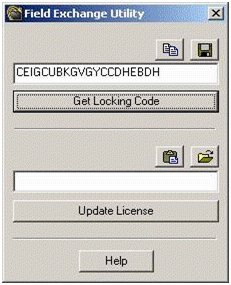
- In order to receive a new license code, please run FieldExUtil.exe program to generate a locking code. FieldExUtil.exe is located on the program CD under Sentinel Driver\Field Exchange Utility directory. This utility is also available from our website at Useful Downloads under “Field Exchange Utility”. Run FieldExUtil.exe program and click on "Get Locking Code" button. Use "Copy to Clipboard" button above the locking code text box to copy the locking code and paste it in an email or use "Save Locking Code to File" button to save locking code to a file and email the file to us. NOTE: Please do not close the program, as we will send you a license code for you to update your key.
- Once you have received the license code from us, please copy and paste the license code in the text box above the “Update License” button. If the license code update process is successful, you should see the following dialog box.
This obscure message indicates a graphics conflict on your system. With INTEGRATED programs it is usually a conflict with NetMeeting running in the background - often without the user being aware of it. The problem can be solved with this procedure:
- Right-click on your desktop and select New>Shortcut from the popup menu
- Set the target as the file IES.exe in your IES program folder. By default this should be in either C:Program Files\IES or C:Program Files (x86)\IES (the latter if you have a 32 bit version install on 64 bit Windows).
- Right click on the new shortcut for your IES program. A menu will pop up.
- At the bottom of the popup menu is "Properties" - left click on that.
- In the dialog box that opens up go into the "Target" location which will have the location for IES.exe and modify it to read IES.exe -g 0 then apply the settings
- This switch indicates that your program should use graphics mode "0". This doesn't exist, and the program will instead search for a safe mode itself.
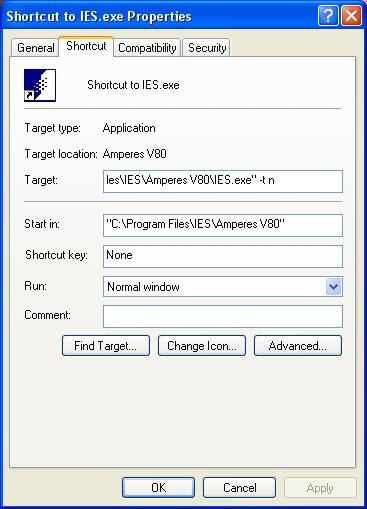
Network versions of INTEGRATED software periodically need to verify the license with the server. In case of short-term network problems there is a wait period before it will interrupt analysis to give a license error. Likewise the server expects to hear regularly from programs it has assigned a license. After a certain time-out period the license can be claimed by other programs. To control these time periods use a -t switch in the program shortcut. To set this switch:
- point your mouse at the normal short-cut
- instead of left-clicking, right-click
- from the pop-up menu choose Properties
- in the Target box click at the end of the progam path ...\ProgramName.exe
- add the switch so the location now looks like ...\ProgramName.exe -t integer
The integer given is your requested time-out period in 10 minutes increments. For example, for "-t 4", the time-out period will be 40 minutes.
Graphics problems are usually related to OpenGL, quite often a bug in your video card driver. Most graphics problems can be solved by forcing a different graphics mode for our software than what is run by default on your desktop.
- Right-click on your desktop and select New>Shortcut from the popup menu
- Set the target as the file IES.exe in your IES program folder. By default, this should be in C:\Program Files\IES folder.
- Right click on the new shortcut for your IES program. A menu will pop up.
- At the bottom of the popup menu is "Properties" - left click on that.
- In the dialog box that opens up go into the "Target" location which will have the location for IES.exe and modify it to read IES.exe -g 0 then apply the settings
- This switch indicates that your program should use graphics mode "0". This doesn't exist, and the program will instead search for a safe mode itself.
Integrated Engineering Software (INTEGRATED) is a research and development organization specializing in BEM-based CAE solutions. INTEGRATED is an established leader in CAE solutions. Started in 1984, INTEGRATED has developed an extensive line of 2D and 3D CAE tools with proven simulation results covering electromagnetic, thermal and particle trajectory applications. INTEGRATED delivers exceptional CAE software tools available on the PC running under Windows 7, Windows 8 and Windows 10. INTEGRATED backs their programs with world class customer service. Live Demos are available.
Most of the time it is easiest to draw a model using a 2D cross-section on a 2D plane, then extruding the model into other directions in 3D mode. Starting with version 6.0 many planes are available for 2D drawing and surfaces drawn on them are automatically recognized in 3D. Some of the commands that you may find useful during your 3D model construction are: MERGE and VISIBILITY. MERGE command enables you to: model a part of your geometry, save it, and later to merge with other parts to create your final model. The VISIBILITY command enables you to make part of your displayed geometry temporary invisible. This allows you to focus on the part of the model you want to concentrate on. To reduce model design and analysis time significantly the symmetry and periodic features are of great benefit. The "Symmetric" and "Periodic" commands are helpful in reducing the geometry size if your model contains symmetry or periodicity.
In recent years, INTEGRATED has pushed ahead with 64-bit processing and then with strategically rewriting more of the time-critical parts of the 3D software to enable multithreading (use of more than one processor core at a time). At the same time, computer manufacturers have made large amounts of memory and multiple processor cores quite affordable. As a result, many users have found dramatic improvements in the solving speed for their most difficult problem. However, the exact speed improvement is dependent on many factors and it is not always clear which factors will be most significant for a given type of simulation. INTEGRATED has previously presented benchmarks for 32 versus 64-bit computing and the effect of the amount of RAM. We are now conducting a much larger study comparing these and number of Processor Cores. In this article we present some preliminary results. The graph below shows the effect of solving a single standard problem under a variety of configurations for a 64 bit Windows 7 system. The hardware has 32 GB of RAM and 2 quad core processors. These were selectively reduced under the Windows Advanced Boot options to study the trends with everything else fixed. COULOMB reported that it requires 6 GB of memory in order to solve the selected problem.
Notice that there is an almost monotonic trend of solving faster as the amount of RAM or the number of processor cores is increased. As earlier benchmarks already showed, there is an especially big improvement as the amount of RAM approaches the reported amount of memory COULOMB reports needing, but we can also see in these graphs that the speed improvement is more substantial when both the number of cores and the amount of RAM is increased than when either is increased alone:
- With a small amount of RAM, 8 processors only solves 30% faster than one processor. With lots of RAM 8 processors solves 4x faster than one processor
- With one processor increasing the RAM produces a speed increase of about 30%. With 8 processors increasing the RAM produces a speed increase of about 4x.
NOTE:the terms "small" or "large" are used deliberately here to emphasize the principle. What is small or large depends on what amount of memory the INTEGRATED program indicates will be required for the model. Hence, it is impossible to properly gauge the best system without inquiring memory requirements for some sample models.
Qualifiers and Concluding Comments:
This study has been constructed to determine what should be good guiding principles for making hardware choices for use with INTEGRATED 3D software. The exact results will be dependent on the actual program and models, but the principles should be common. The main benefits of the type shown above will be found with the BEM solver in 3D programs. However, the same advancements will continue to be further expanded to other parts of the software in coming versions.
General Recommendations:
- Our programs run on all 64-bit versions of Windows 10 and Windows 11.
- At least 4 GB of memory is recommended.
- As we use OpenGL for rendering geometry, a graphics card is required for 3D programs.
2D Programs:
- Typical models run quickly on a minimum of 4 GB RAM.
- Although single processor machines are often adequate, the software will make full use of multi-processor and multi-core machines.
3D Programs:
- Typical models run quickly on a minimum of 16 GB RAM. Larger models run faster and better as more RAM is used.
- Multi-core and multi-processor systems are highly suited as 3D programs are multi-threaded.
Available RAM versus Problem Size
For small problems the processor speed is the biggest consideration for calculations. If your processor works at twice the speed the problem will be solved in half the time. Get an approximate total speed by multiply clock speed by the number of cores.
Memory required is roughly proportional to the number of calculations needed to solver, so over a wide range of operation it can be used to estimated total solution time. For example, if you solve a model in 5 minutes, then the next model reports needing twice as much memory, it will probably take about 10 minutes.
Memory management progressively becomes a bigger and bigger consideration when the problem becomes larger and larger. If the memory needed to solve is larger than available RAM – then most of the problem is being swapped back and forth between RAM and the hard disk as the problem proceeds. The efficiency of this process becomes the biggest single factor in the speed of solving large problems. Since this is managed by Windows itself – taking account of other processes also running – we can do very little to help you optimize further from within our software, but can offer the following advice regarding the system setup:
- Determine the size of problems you will be solving. This is reported in the Message Area as required disk space when the BEM solver begins. It is also reported for the existing element distribution from the menu Solution>Elements>Problem Size.
- The importance of getting as much RAM as needed is illustrated by the benchmark results below for a COULOMB™ problem run with different number numbers of elements. The more elements the more accurate the solution, but the more memory that is required. Up to a couple of GB of RAM there are overheads setting up the solution so the solver speed seems low, but it is also only a few seconds in total so speed is not normally considered an issue. For problem size between 2 and 50 GB the solving takes a few minute. 50 GB take about 10 minutes (that is, a speed of about 5 GB/minute). However, since the system has 64 GB, and Windows and other programs use several GB, above 50 GB the speed can drop substantially as COULOMB™ has to start managing memory by read/write to the hard drive. The green line shows where the problem size matches the total system RAM. This is already slower due to not having enough RAM available, and it slows down even more beyond that. The 120 GB solution took 50 minutes.
-
When buying a system for analysis the reported memory for the models you have been solving is thus a guide to how much RAM you should be getting on the system.
Comparison of solution times for a non-linear 3D magnetic model requiring 6 GB memory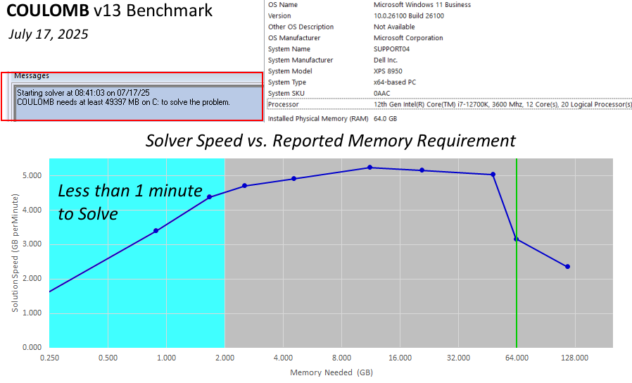
- 2 hard drives: When choosing hard disk features access time is clearly important. You can set up the locations of the scratch files from Utilities>Settings. Out of various configurations we tested, this was the single most important factor in performing faster analyses when the memory required exceeded available RAM.
- RAID ARRAY: using a RAID array lets you use multiple disks as a single drive letter, but will manage the access very efficiently. We configure our own systems such that IES software is installed on d: (a RAID array) with the program and scratch files using d:. For more generic information about configuring a RAID array on your computer, check HOW TO: Establish a Striped Volume (RAID 0) in Windows Server 2003 (Microsoft Knowledge Base).
Our software is written to run on Windows operating systems including Windows 10 and Windows 11.
Heat and resulting temperature distribution always has to be a Finite Element Solution. But if you just want to calculate power loss distribution, that can be done using BEM.
Yes, there are two ways. You can assign a constant volume current and then calculate the power loss, or you can use eddy current windings with a voltage source and obtain the resistance from the winding current.
Yes, but it depends on the thickness of the metal switchgear and how big the overall system is. Because it can take up quite a bit of computer time, you have to deal with it on a case to case basis.
For the electromagnetic portion of the solution, you can use either the Boundary Element Method (BEM) or the Finite Element Method (FEM) if you are performing a time harmonic (phasor) simulation. If you are performing an electromagnetic transient, the Finite Element Method must be used. For thermal analysis (static or transient), only the Finite Element Method can be used.
Although this might indicate a bad solution, it usually is an artifact of the nature of the contour plot which is exagerated by the plot being too coarse with respect to the geometric detail. To illustrate the nature of contour plots and artifacts such as this, consider the electrode (light yellow area bounded by black lines) below. To generate a voltage contour plot over an area surrounding the electrode, a grid is set up and the voltage is calculated at the cross-points of the grid. The points closest to the electrode are indicated in red as V1-V9:
In total the sampled points will produce voltage in the range Vmin to Vmax. Now, we request some number of contours, and hence assign contours to the levels Vmin + n*(Vmax - Vmin)/number Suppose that process results in the contour which will be colored blue being assigned to a voltage V' which is close to the voltage of the electrode shown. What we do to plot the blue contour is to interpolate between neighboring sampled points and put a blue dot wherever a value of V' is achieved.
Next, we connect-the-dots with blue lines.
You can see that this process will produce contour plots, but that they will intrinsically cross the electrode boundaries in a case like that shown above no matter how accurately the values are obtained at V1..V9. However, by making a finer density plot, there will be more detail around the electrode and the contours will wrap better around them. In INTEGRATED software you can make finer density plots by either using the Coarse/Medium... switch, or by making a more local plot on any given setting. In fact, our Coarse/Medium/Fine/Very Fine options are a bit more intelligent than this explanation. You will note that they take longer to set up the points than the User Grid option, because they do attempt to locate the points intelligently with respect to surfaces (i.e. it is taking extra time to adjust positions in a non-uniform mesh). This is one aspect of the software that tends to improve from version to version. However, no matter how sophisticated this routine becomes, if there are not sufficient sampled points then one thing or another will look odd in a contour plot. Also note that, you cannot tell by looking at a contour plot where the sampled points are, only where the vertices obtained by interpolation are.
Background on contour plots
When we make a contour plot we set up a grid of x,y,z coordinates and calculate the field at those points. We then do interpolations to sketch out the lines that get plotted and displayed on the screen. The interpolations are simply a series of straight lines that connect points of similar values. There will be cases where points are near corners and that will mean interpolations might actually cut through a material but this is simply a display issue and does not mean you have a bad solution. You can improve this particular problem by choosing to do a contour plot with a higher density (Medium instead of Coarse or Very Fine instead of Fine, etc.) This includes the ability to choose a user defined grid where you can input the number of points in a Row, Column format. If you are calculating the field near a source of high field value (sharp corner, etc.) then the maximum field value will vary as you change either the size of your contour plot or the density of the plot. This happens because the coordinates where the field is calculated for a contour plot is somewhat arbitrary so the maximum value displayed by the contour plot will depend purely on how close one of the points used for the contour plot comes to the maximum value. The best thing that you can do is set the maximum value to be a bit lower than the value reported by the program and see how much of the contour plot disappears. If nothing noticeable changes then you are probably seeing a singularity (e.g. corner) that is giving a high field value, if a section of the contour plot disappears then you are seeing real values of the field that you would be concerned about in a design. A better way to look at the field values from geometry is to do a graph along a line from one point in space to another. You can vary the number of points you are creating your graph from and it is much easier to see a continually varying result. It also happens to generate results faster.
A Note on FEM in cases such as these:
One of the drawbacks of FEM is that it only calculates the voltage (or in magnetics the magnetic (or vector) potential) at particular points in space and then interpolates everything from those points. This can cause interpolation errors and can also cause rippling in the field plots, as you need to differentiate discrete potential data to get the field. The difference between the interpolation errors in FEM and the ones in BEM are that FEM interpolation errors are real and will affect your solution whereas the ones in BEM are only there for displaying things like contours. If you query a point in space in FEM the program will interpolate from known points and produce an approximate answer based on solved points around the point that you want. In BEM if you query a point in space the value at that exact point will be calculated and no interpolation error would result. It is because of this fact that BEM is so highly valued for charged particle optics packages. One other result of interpolations done with FEM results is that they tend to artificially suppress field values at corners because the high field values get missed. The "maximum" is thus a feature of the FEM mesh rather than a true physical aspect of the model. In BEM no such artificial limits occur. The user has greater control based on the solution being more correct to theoretical result for the given geometry. Thus, the user can intelligently find the maximum field based on either rounding the geometry, or by ignoring the results at locations unrealistically close to the corner when analyzing. For more information on the modeling issues involved, see: Benchmark Problem for Simulating Electric Fields Near Sharp Corners and Benchmark Problem for Simulating Electric Fields Near Triple Junctions
In streamlines, the test charge used has no mass, or velocity. This means it follows the path of the electric field. Effectively what you should end up with is a limited version of the E-field. To calculate the resultant curves, Coulombs law is used. Streamlines can be drawn off of a voltage potential, or from a point in space. When drawn from a voltage potential, the streamlines will be placed leaving from both sides. From a point in space, the streamline will travel in the direction of increasing or decreasing field. For the trajectories, a particle is used possessing charge, mass, and velocity. Thus the resultant path does not follow the electric field, but rather a path dictated by F = m a, where the electric field acts on the particle to slowly change its direction. Particles are launched with a user specified velocity, and direction.
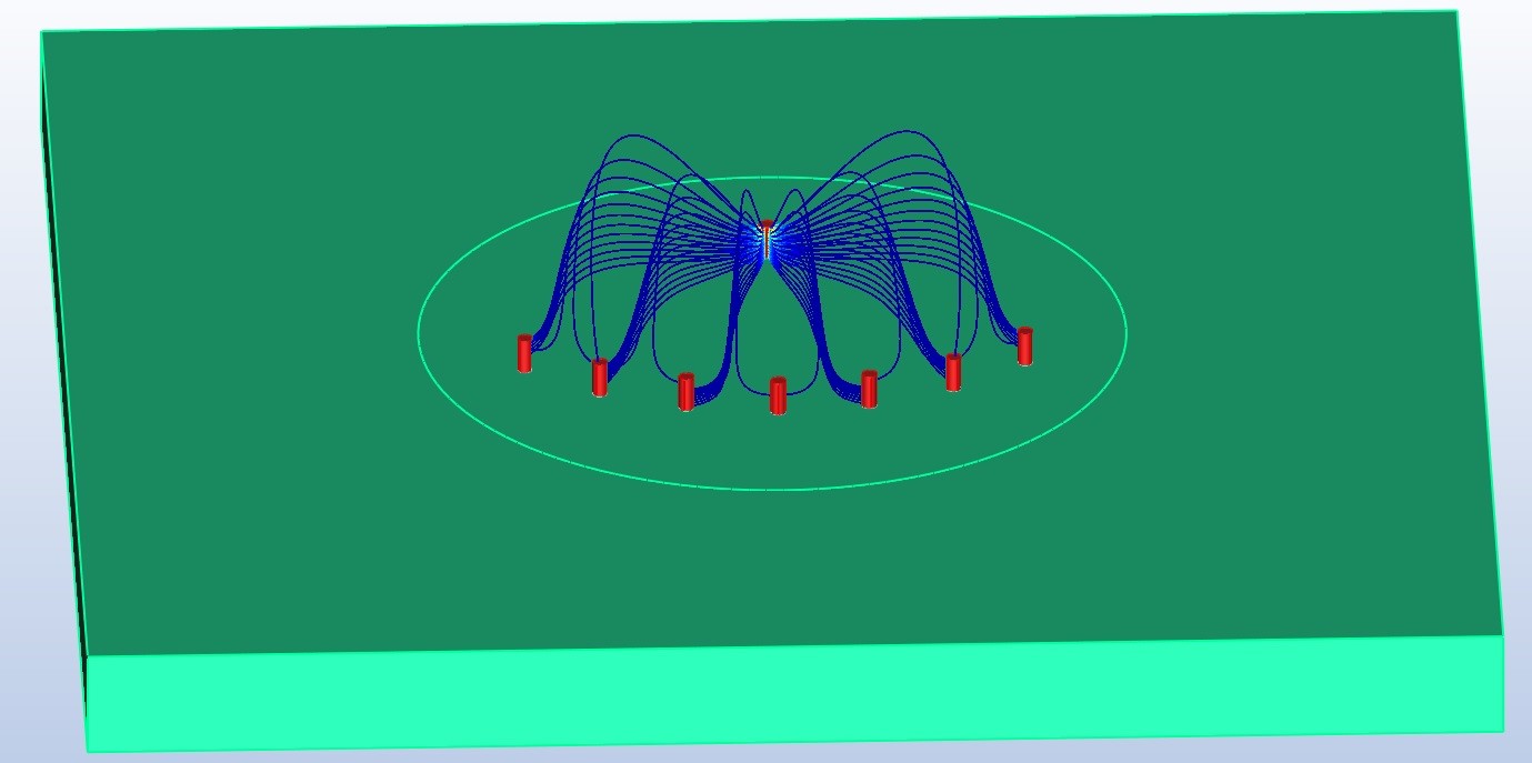
Streamlines originating from one source and terminating at multiple grounds modeled on a PCB substrate in Coulomb 3D
For a 2D model, the total loss is given in W/m and torque in N*m per m. As the result is assumed to be continuous in the direction perpendicular to the two-dimensional model, the total loss in W or the total torque N*m is obtained by multiplying the loss in W/m or the torque in N*m per m by the motor's length in metres.
INTEGRATED's CAE tools create two temporary scratch files during analysis. Prior to performing an analysis you can check the scratch file size by using the command ProblemSize under the Element submenu. This command displays the size of each scratch files in Mega bytes. The size is related to the number of elements in your model. The location of these scratch files can be set (for example to different disk drives). In version 6.0 and older Choose File>DirectorySetup to set directories for the databases, and scratch files. In version 6.1 and newer choose Utilities>Settings then choose Files in the Application Objects Tab. From there you will be able to change the location.
MAGNETO has the ability to input a magnetic loss curve in the Material Table and then assign the material to the model's geometry. The magnetic loss curve combines hysteresis loss and lamination loss (eddy current losses in the laminations) information. These loss curves are available from the material supplier. The software requires that you place subareas in regions with lossy materials for the total loss calculation to solve the loss density over the entire region. If you are only interested in power loss density, you can leave the subareas out.
As a rule of thumb, boundary elements should not be longer then 10x the distance to the nearest element with similar orientation. This applies to surfaces that have long narrow regions, such as motor air gaps and parallel plate capacitors. As well, the number of boundary elements should be increased where the field changes rapidly. See Online Help for more details
Unlike the Boundary Element Method (BEM), the Finite Element Method (FEM) is a numerical technique for solving models in differential form. For a given design, the FEM requires the entire design, including the surrounding region, to be modeled with finite elements. A system of linear equations is generated to calculate the potential (scalar or vector) at the nodes of each element. Therefore, the basic difference between these two techniques is the fact that BEM only needs to solve the unknowns on the boundaries, whereas FEM solves for a chosen region of space and requires a boundary condition bounding that region. BEM and FEM have become the two dominant numerical techniques in computer-aided engineering (CAE). Both techniques have merits and restrictions. In fact, Integrated Engineering Software uses both methods as well as the Hybrid Method. Our conclusion is that BEM is overall the superior solution technique for electromagnetic designs. Historically we have therefore focussed on BEM and have been strongly associated with it in the marketplace.
The major advantages of BEM
Ease of Use
Unlike FEM, which must use a 3D finite element mesh in the whole space, BEM uses only 2D elements on the surfaces which are the material interfaces or assigned boundary conditions. Therefore, users can set up a problem quickly and easily. Since only elements on interfaces are involved in the solution procedure, problem modifications are also easy. For example, in motor design optimization, solutions are required for different rotor positions. Using BEM software, only one boundary element distribution is necessary to solve all the rotor positions, and no element reassignments are required. With FEM software, finite elements in the whole space must be re-generated for every new rotor position. Complete 3D Finite Element Meshes are impossible to visually represent and comprehend on a 2D drawing.
More accurate results
BEM allows all field variables at any point in space to be obtained very accurately. Also, the results are more precise because the integration operation is smoother, making BEM inherently more accurate than FEM's differentiation operation. Moreover, the unknown variables used in INTEGRATED's software are the equivalent currents or equivalent charges. These variables have real physical meanings. By using these physical variables, global quantities such as forces, torque, stored energy, inductance, and capacitance among others can be accurately obtained through some very simple methods.
Superior analysis of open boundary problems
The analysis of unbounded structures (e.g. electromagnetic fields exterior to an electric motor) can be solved by BEM without any additional effort because the exterior field is calculated the same way as the interior field. The field at any point in space can be calculated (even at infinity). Therefore, for any closed or open boundary problem INTEGRATED's software users need only to deal with real geometry boundaries. In contrast, open boundary problems are problematic for FEM since artificial boundaries, which are far away from the real structure, must be used. How to determine these artificial boundaries becomes a major difficulty for FEM-based software users. Since most electromagnetic field problems are associated with open boundary structures, BEM naturally becomes the best method for general field problems.
BEM solves non-linear problems
BEM can readily solve non-linear problems. Many people, including some who are quite knowledgeable about BEM initially, believed that BEM could not solve non-linear problems. However, the truth is that not many people know how to use BEM for solutions to non-linear problems. Later on we will discuss in more detail how BEM is used to solve non-linear problems. For now it is sufficient to point out that BEM routinely solves non-linear problems.
BEM does error analysis
From Green's theorem one can show that if and only if the solution satisfies the boundary conditions on all the boundaries, the result at any point in the solution space obtained from the variables on the boundaries is correct. Therefore, after solving a problem with certain element distribution, users can perform an error analysis by checking the boundary conditions along the boundaries. One can improve the solution by simply adding more elements on the boundary where a large error has been found. This is based on the fact that the largest errors occur on the boundary, and that for the fields in a region the largest contributors are the elements close to the region. We have an error detection command in all of our 2D/RS software.
Advantages of FEM
While BEM can solve nonlinear problems, the nonlinear contribution requires a volume mesh. Putting a volume mesh in begins to diminish the benefits of BEM listed above. In fact, for a saturating nonlinear magnetic problem, the saturatation characteristic is best solved with FEM. Also, the BEM benefit of solving open regions very well is not always relevant.
Suppose you have recorded a series of batch files: batch1.txt, batch2.txt, batch3.txt... You can launch these individually, or using a "Batch in Batch" (BIB) file. For example, using the above batch files make up a text file called "batch.bib" consisting of the following lines:
- batch1.txt
- batch2.txt
- batch3.txt
- batch4.txt
- ...
The Boundary Element Method (BEM) is a numerical technique for solving Boundary Integral Equations. This is our default method for solving as we find it to be the fastest and most accurate general purpose solution method. From version 6.1 and higher, users have other options (e.g. a Finite/Boundary Element hybrid in 2D programs) to deal with specific issues since no single solution method is the best for every problem type. In the BEM technique, electromagnetic, thermal and structural phenomena are mathematically described by appropriate equation systems (e.g. Maxwell's equations for electromagnetics ) in integral form. Enforcing the boundary conditions along the material interfaces allows one to obtain a set of boundary integral equations with the unknowns as the equivalent sources or field variables along the interfaces. One may then discretize the boundaries to boundary elements, represent the unknowns on elements, and obtain a system of linear equations. In this way BEM solves a given problem. All field variables at any point in space may be obtained by performing integrations associated with the equivalent sources or fields on the boundaries.
From version 5.2 upwards IES is using OpenGL for rendering the model display area. This has had many benefits for providing better model and analysis display, however, OpenGL does require more than 256 colors. The MS Terminal Server window only uses 256 colors, hence, it will be very difficult to obtain meaningful displays. One option available is to use the -g switch to override the default video display setting when calling your IES program. This way you can at least get the video mode best suited to running your program in the terminal window. We have found best results with video mode 11 on our own systems. So for example, the shortcut to AMPERES can be modified to
- amperes -g 11
This works either by modifying the shortcut (keeping path information the same) or by creating a DOS batch file with the above content to start the program. Video mode 11 displays the workspace on a black background with dark red lines and bright dots. In shaded modes the dark red is dithered. This provides some model viewing, but it is still recommended that you do your basic set-up work on your desktop, then run from a terminal window for solving and possibly some basic post-processing (finding forces, plotting lines). If video mode 11 doesn't work as described for you, or you would like to experiment - get GLView here and run it in the terminal window. The mode numbers which indicate OpenGL and provide the nicest display of a rotating cube are the ones to use with your IES program.
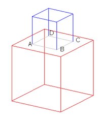
Consider a simple example of a small cube placed over a big cube. If these two volumes are in proper contact, they would have an unique surface in common. In the Fig. 1a shown below, it appears that the two volumes are in proper contact, but they are not. The easiest way to verify whether these two volumes are in contact or not is, assign different materials to these volumes with the help of the command “Assign” of the “Physics\Material Table” dialog box. See that the color of the each material is distantly different from the other. Observe the color of the edges of the common surface ABCD in Fig. 1b. It is blue which is the same color of the other edges of the small cube. Had the surface ABCD been a proper common surface to both the volumes, the color of its edges would have been light gray which is neither the color of the small cube nor the big cube. Since the color of the edges of the surface ABCD is blue, the geometry shown in Fig. 1 is not valid for the field analysis.
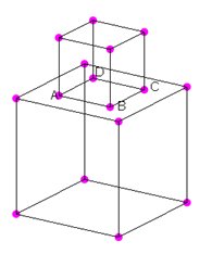
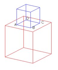
The geometry shown in Fig. 2 and Fig. 3 are valid because the color of the edges of the contacting surface ABCD is light gray. You may choose any one of these two valid geometries for the field analysis.

Whether you import a model from a CAD package or draw it in IES software, it is important that the drawing be physically realistic. Many things that are easy to draw, or which may be drawn to facilitate manufacturing (e.g. a cylinder "force-fit" to a hole, being slightly larger than the hole it is being inserted into), are not physically possible, hence they will adversely affect attempts to use the drawing for engineering analysis. It is less work to have such problems addressed by training the person doing the drawings than it is to try to modify the drawings when they are completed. One of the more subtle problems that comes up is "overlapping surfaces" - illustrated to the right. On top is a cylinder of copper, underneath is a block of steel. Where they meet, there is physically only a single interface. As shown in blue on the left, there is essentially a hole in the top surface of the steel block, and this hole is the interface between the two.
Consider what would happen if the drawing was made by constructing a block, then constructing a cylinder. As shown in blue on the right, the whole top surface would be one surface. Problems that result include that the boundary condition for the solution will have this as either a steel/air or a steel/copper interface - not as a combination of both. Even if the elements were to individually check what material is on each side - there would be many elements crossing the boundary of the small circle - hence the boundary would effectively become very coarse. Since there can only be a single surface between the copper and steel, and since this surface is distinct from the rest of the top of the steel block - a model for CAE purposes needs to be drawn that way. The rest of this FAQ entry addresses how to do this in version 6.0 of IES 3D software. The principles given here can be applied to drawing in various CAD packages for those customers wishing to use our direct CAD import feature.
While recognizing holes in surfaces is very difficult in 3D, it is relatively simple in 2D. Hence, the first step is to draw the intersecting surfaces using the 2D mode. After entering the 2D mode you draw a rectangle with a circle inside it. The fact that the circle is a hole in the rectangle is automatically recognized.
Now when you switch to 3D mode the software will recognize the 2D region with a hole as a 3D surface with a hole. The hole will also be defined as a surface (though in some cases it might be convenient to undefine it).
From this point the basic problem of overlapping surfaces is solved and there are many drawing options. One simple method is to sweep (extrude) the circle upwards into the cylinder, and the top surface, plus the hole in it downwards. This produces 3 volumes as shown. In fact, for the similar problem of a copper rod sticking though a steel block, this is exactly the geometry you want. However, for the stated problem the cylindrical volume within the steel might be deemed a nuisance since it requires an extra step in operations where the steel volume is being selected. If so, it can be deleted as follows:
In IES software all you need to do is delete the 2 segments that define the circular bottom of the volume and the side length. This breaks both the volume and bottom surface of the steel (since you have removed part of the boundaries for each). Redefine the bottom surface and you can now redefine the volume as well. You have now created the physically correct volumes and surfaces, and you can assign materials to the volumes - and any other appropriate physical parameters.
In version 6.0 of our 3D programs we introduced NURBS for easier definition of more general surfaces. However, we also still permit users to define surfaces from a Coons Patch routine based on the bounding segments of the surface. A basic description of each is given in Advantages of NURBS in CAE Modeling - this particularly demonstrates the difference in describing curved surfaces. The only case of creating geometry where you need to be concerned about the limitations of the Coons Patch is when you are using the "Define Surface" tool rather than sweeping/extruding, using the 2D mode, or using the primitives to create surfaces.


To the left is an example of a surface that works well as a Coons Patch. If you can readily draw a 3 or 4 sided figure and put a grid across corresponding sides to make the surface, it will work. To the right is a surface that will be tricky, if possible at all to make work as a good single surface. To see this, look at the meshes obtained if one chooses various groupings of the sides.
This skinny "L" shape was deliberately chosen for the fact that while it seems a simple enough shape, the surface mesh clearly doesn't stay within the presumed limits. The math of the Coons patch simply isn't that sophisticated. It is recommended that you avoid interior angles greater than 180 degrees. Our old method of fixing these problems is shown to the left. Our new method is shown to the right. In this case the surface was drawn on a 2D plane, or displayed on a 2D plane after drawing so that all closed regions would be recognized. These are then interpreted as 3D surfaces when you switch to 3D mode. Now it isn't possible to draw quadrilateral elements, but the triangular elements mesh most surfaces better and show no problem with the surfaces that are properly recognized rather than defined from the Coon's Patch.
Another tricky aspect of the Coons Patch is surfaces containing holes. For more on this see the following question: How can I draw a model without overlapping surfaces?
The periodic modeling features allow customers to take advantage of linear or angular periodic properties of their devices by modeling only the periodic portion of the device. This capability greatly simplifies model design time and significantly reduces model analysis time by up to 90% without sacrificing accuracy.
- Step 1: Create the model’s periodic portion by creating a partial CAD model with the appropriate physical properties assigned.
- Step 2: Assign boundary elements to all surfaces except those shared with the other periodic sections (not modeled).
- Step 3: Select whether or not the design is linear or angular periodic, which axis (X,Y,Z) the model is periodic on and whether the design is anti-periodic (alternating sources direction voltage, currents or magnets) or just periodic. Finally, the designer must specify the number of periodic sections. For linear periodic models you must provide the number of sections modeled, the total number of sections in the full design and the length of the complete design. For angular periodic models, only the number of sections in the full design are required.
- Step 4: Periodic analysis is then performed. Periodic analysis solves just the periodic structure, saving significant analysis time.
- Step 5: Review complete results for the entire structure (e.g. total torque, magnetic flux, capacitance, etc.)
There are two reasons you may see the error message shown to the right:
- You have not yet configured the Pro/E environment variable. For a description of how to do this, see How do I use the direct import from PRO-E?.
- You may be hitting a Pro-E bug which causes CAD links to "time-out" on January 10, 2004. You can download a patch to fix this bug from http://www.ptc.com/go/timeout/
The import from PRO-E requires an environment variable to be set up.
- from your desktop Start menu choose Control Panel
- click on the System icon
- Choose the Environment Variables tab (depending on your Windows version this may be under "Advanced").
- Setup a new variable with properties as shown below, with a value appropriate to your program version and location. The variable value should be the full path (e.g. c:\Program Files\...) pointing to the PRO-E executable file pro_comm_msg.exe
The first time you use the import you will first need to choose a Pro-E version.
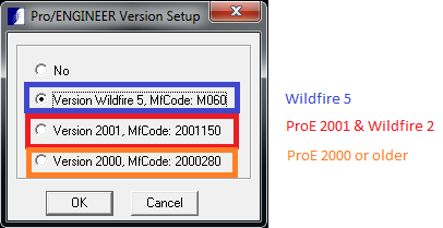
The reason is the PRO-E link is version dependent. So you choose according to whether your release is before or after this. Using the Link Once the Environment Variable has been set up and the version is chosen, you are able to start PRO-E and your IES 3D software. Now, open a model in PRO-E. Then selecting File>Import>PRO-E will import the model from PRO-E. Also see: Why do I get an error message Unable to Connect to Pro/Engineer?
The import from SDRC IDEAS requires an intermediate program to be launched from the SDRC "Additional Applications" launcher. The icon circled to the left will bring up the dialog box shown. Type in the program name as shown, then within your IES software chooseFile>Import>SDRC IDEAS and select in SDRC-E the part to import. After each part is imported, your IES program will prompt you to determine whether to import another part
Export Options from SolidWorks save as dialog box.
Starting with version 6.0, Integrated Engineering Software (INTEGRATED) tools have a direct memory access to major CAD packages. This makes a more accurate and seamless import than using CAD file exchange formats. With the model open in the CAD package, look down the File menu for Import and choose your CAD program from the list. Note that Pro-E and SDRC require some additional setup as outlined in
INTEGRATED's CAE tools also accept IGES, DXF, STEP and SAT format files. The IGES, DXF, STEP and SAT file formats are standard CAD design file transfer formats. All major CAD systems provided one or more formats as an output option. IES imports IGES, DXF, STEP and SAT file formats and provides tools to edit the imported CAD designs. In addition, each of INTEGRATED's CAE tools come with complete built-in CAD toolset.
In version 6.1 & 6.2 the menu Physics>Material Tablebrings up a small dialog box with options to Modify, Create, Delete, Assign or Inquire Materials. The Modify and Create options open up a Material Editor dialog box where you can choose the material property you wish to modify and (if they are characterized by a single number) type in a new value. A nonlinear material or a permanent magnet is characterized by more numbers and requires either clicking to edit the data in AutoGraph or loading a new material. See the video Loading a Nonlinear Magnetic Material. When using AutoGraph to edit a material remember to click Apply in the Material Editor before closing Autograph. Many customers prefer to open an existing material file and use it as a template. They change the name, paste data in from a spreadsheet, and save under a new name to be loaded as shown in the video.
1-Phasor mode
In Phasor mode the dielectric constant is considered to be a complex number consisting: ε = εr*εo + j * σ/ω where: εr = relative permittivity, εo = permittivity of free space σ = electrical conductivity ω = angular frequency = 2πf In most cases, for most materials, either the real or the imaginary part will be orders of magnitude larger than the other at the frequency of operation. If it is the real part that is much larger the material for practical purposes behaves as, and should be modeled as, a perfect insulator. If it is the imaginary part that is much larger, the material is operating as a conductor. For example, a typical "insulator" used in an electric model might have a conductivity of 10-12 /Ω-m and a relative permittivity of 4. Using INTEGRATED's Quick Engineering Tool for Lossy Dielectrics, this produces an imaginary part of the relative permittivity of 0.0003 when the frequency is 60 Hz. In this case it is very accurate to model with the conductivity=0 for faster results.
2-Transient
In the general time dependent case, the response of a model to time varying signal involves movement of charge and changing of polarization. These give rise to the characteristic time responses at various points in the system. In the case of a harmonic signal this can be treated at real and imaginary parts (above), but in general it is simply considered a "transient response". Consider the very simple parallel plate system shown below:
If we monitor the voltage at the interface over time, it will behave the same as this circuit:
The dielectric layer behaves as a resistance in parallel with a capacitance, and the empty space layer behaves as a capacitance. The interface is designated by a node labeled "i". The conductivity was selected so that the INTEGRATED Quick Engineering Tool for Lossy Dielectrics would predict a "time constant" of 0.2 s. An analysis with ELECTRO then determined the following voltage response at the interface:
Note:
- Since the capacitance of the dielectric layer is 3x that of the empty layer, 3/4 of the voltage is across the empty layer when the voltage is first turned on.
- Once the voltage is turned on, charge begins to leak through the material. Over time the voltage across the dielectric is decreased.
- In one time constant (0.2 s) the voltage across the dielectric layer is decreased by a little more than half, but not as much as 1/e. The latter would be the response if the system consisted entirely of the dielectric layer leaking charge. In the whole model ("circuit") the response will be different, but of a similar magnitude. Hence the time constant estimation given INTEGRATED' Quick Engineering Tool for Lossy Dielectrics provides the relevant time frames for setting up transient parameters.
3-Static
Referring to the simple case in section 2 (Transient), a "static" model is actually a transient one of two limits after a DC voltage is turned on: either it is the initial response over times much shorter than the time constant or it is the final state after all transient effects have decayed away. As an example, check the calculator for conductivity=10-15 S/m and relative permittivity=4. The time constant is approximately 10 hours. So if the voltage is turning on an off over a few seconds or minutes, the conductivity is irrelevant. However, if it is turned on and left on for months, the long-term behavior is dominated by the conductivity of the material.
- In the high voltage industry a failure is often found days or weeks after turning equipment on. Due to the high resistivity (low conductivity) of the materials used the time constant may be very long, but the equipment may also be ON continuously for a long time. In this case two analyses are needed for potential high field problems in the materials: a permittivity mode solution for the short term response, and a conductivity mode solution for the long term response. If the transitional states are of interest, those need to be modeled in transient mode.
When using periodic conditions, you should ensure that your model satisfies the following 3 conditions:
- Active geometry does not overlap when it is rotated into position (Overlapping active geometry gives non-physical results).
- Segments with periodic boundary conditions do not contain elements. These boundary conditions define areas where the material is continuous into the next periodic segment.
- The center of the model is located at the origin in 2D or on an axis in 3D.
All INTEGRATED software is designed to exploit periodic conditions in models. Using periodic conditions - force, torque, power, energy, flux linkage, and the magnetic fields are calculated as if the whole geometry is present. By reducing the number of unknowns you need to calculate, you can greatly reduce the time required for simulation. An example of this is a DC motor with 24 slots in the stator and 4 permanent magnets on the rotor. In trial runs, the periodic model took only about a minute, while the non-periodic model took nearly 20 minutes. This increase in time is because the number of calculations required is proportional to the number of elements squared. Thus if your reduce the number of elements to 1/4, you can reduce your simulation time to 1/16 of the original time required. Take special care when assigning periodic conditions to ensure that active geometry does not overlap since overlapping geometry creates conditions that cannot be physically achieved.
Creating a nonlinear material file:
- With a standard text editor create a file in the program directory where the other material files (*.mtl) are located. If you are dealing with a program that does not have a material folder already then it is a good idea to create one.
- Create three columns of numbers using the following format: Point Number X coordinate Y coordinate
- The first nonlinear material point has to be 1 0.0 0.0 unless the material is a permanent magnet. 10-15 points will create a good nonlinear curve. The end point for a 1st quadrant curve takes the slope from the last two points and continues the same slope after the last point.
- If you are making a BH curve and are given the hysteresis loop, use an average of the two paths to define the curve (mean BH curve).
- For permanent magnets, a second quadrant curve is defined and must start at y=0 and end at x=0. At least 3 points are recommended for a straight-line model.
- Save the new material file with the extension *.mtl (no character limit). The material is now defined and ready to be loaded into your model.
Reading and Viewing the new nonlinear material file:
- Before loading in your new material, make sure the units settings are the same as the ones that were used to create the material lists. For example if you used Gauss and Oersted to define the material, then make sure the units are set to Gauss and Oersted in the Utilities> Units Setup window. This information will not be passed in to the program from the file. Instead the program will assume it is reading in whatever units the settings are at.
- To load in your new material open up the materials list and select a material that will not be used in your model. You will replace this material with your new one. Click on File>Load Nonlinear Curve and select your new material.
- When you load in this new material the name will not change. You must do this and click on the Apply button.
- Confirm the curve looks correct by opening up the materials list and clicking on the nonlinear curve editor as the points entered are defining a spline-fitted curve.
Magnetic materials generally have a nonlinear and history dependent B-H magnetization characteristic, as illustrated in the generic hysteresis curve to the right. However, for practical purposes magnetic materials can usually be considered as one of two types:
- Red curve: ferromagnets (e.g. steels), paramagnets, and diamagnets
- Blue curve: permanent magnets
The Material Editor screen capture to the left shows the material types for "Parameter: Permeability" corresponding to the descriptions above. Ferromagnets can be Linear (permeability only) or Nonlinear (B-H magnetization curve). Paramagnets and diamagnets are linear. They are specified by relative permeability or susceptibility. The input boxes are linked by formula as: χ = µr – 1 and µr = χ + 1
Many materials cross the second quadrant reversibly along a straight line. These can be modeled as shown to the right by inputting the axis points Br and Hc. In some other cases the behavior is linear and reversible enough over the range of operation that the option shown to the right still works. In other cases the B-H characteristic may show significant curvature, but the behavior is still essentially reversible. Then the Nonlinear Permanent Magnet type works in a straightforward way. For some materials and applications, irreversibility is a significant consideration. For example, for Alnico 5 shown below:
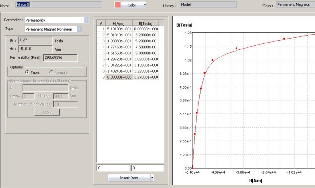
Over a small range of operation near H=0 the curve will retrace as H is increased and decreased. However, by the curve of the knee the magnet is changing material properties. If H becomes so negative that the blue point is reached, then as H changes between this value and zero the magnet operates along the blue line shown. Likewise if H becomes so low that the green dot is reached, then the magnet operates along the green line. With such materials, the analysis necessarily involves several steps because the range over which the magnet is used will affect the appropriate material curve.
- Step 1: Using the supplied data (pink shown below) analyze the model over the range of operation to determine the largest (negative) values for H.
- Step 2: Replace the data curve, or define a new material, with the red curve shown below, corresponding to the correct characteristic for the material after a cycle through the range of operation for the device.
Note the data to the left of the operating range is irrelevant. Hence, it is common to define the material as linear with a selected Br , Hc which produce the correct behavior over the range of operation. A supplied magnet will generally have been transported in an open circuit (no ferromagnetic return path) condition. This should be modeled as one of the scenarios for determining the true operating state. A supplied magnet may have been "stabilized". That is, it may have been deliberately demagnetized to a state which will be reversible under a large range of operation. In this case the B-H data entered should not be the general data for the material, but should be provided by the supplier to specify the state after stabilization.
INTEGRATED offers two licensing options: virtual keys and Thales hardware dongles. Virtual keys require only an internet connection, eliminating the need for hardware dongles. Hardware dongles are USB devices that track the program ID and the number of programs being run. Users have the freedom to install the software on as many computers as they wish. The software will only run at any given time on the computer enabled by the virtual key or the dongle. Depending on your needs, you may choose a stand-alone dongle, which you physically move from computer to computer to change which has the license, or a network dongle, where the dongle is installed on a single computer that controls the license usage on other computers. Note: The virtual key option is for stand-alone use only.
The error message suggests that your firewall may be replacing our digital certificate with your company’s own certificate. Our program communicates with our server using messages encrypted with our company’s digital certificate. Your firewall appears to have intercepted these messages and re-encrypted them with your company’s digital certificate, a process known as SSL inspection. Our program will reject the messages because they are no longer signed with our company’s certificate.
To prevent this from happening, please make an exception in your firewall settings to allow messages between our server (https://bd73dsl.integratedsoft.com) and our program to pass through unmodified.
Before proceeding, ensure the key is properly plugged into the computer’s USB port. The light on the key should be ON. If the light is not ON, try another USB port or contact INTEGRATED Support.
For SK4 series keys, the most common reason for this issue is the absence of the Sentinel Driver. Visit the Useful Downloads page and download the Sentinel System Driver if you have an SK4 series key.
If you have an NPU series network key and are installing it on the license server, download the Sentinel Protection Installer. If you are unsure whether the Sentinel Driver is installed correctly, download the Sentinel Medic program from the download page. The Sentinel Medic should confirm the presence of a key and display the installed driver version.
Note: SK5 series keys do not require a driver.
Another common problem is a mismatch between the key number and the program installation. The error message should indicate the expected key number, which should be printed on the key label. If the number on the key label matches the error message and the latest Sentinel Driver is installed and verified by the Sentinel Medic program, the key itself may be corrupted and require replacement. INTEGRATED Support can assist in verifying this.
In rare cases, the driver is installed but the key is still not recognized. This may be due to port contention, where another software is using the same port as the key. For SK4 and NPU series keys, the ports are 6001 and 6002. Ensure these ports are not used by other software.
The network program periodically contacts the license server to let the license server know that it is still running. You can control the amount of time the license server is expected to hear from the client. The default period is 10 minutes. If the license server has not heard from the client during this period, the license is returned to the license server. You can create a short-cut for the program and edit the "Target" box in the short-cut. Add the following program argument after the executable name: -t n where n is a positive integer in multiple of 10 minutes. For example, n=6 is equal to 60 minutes.
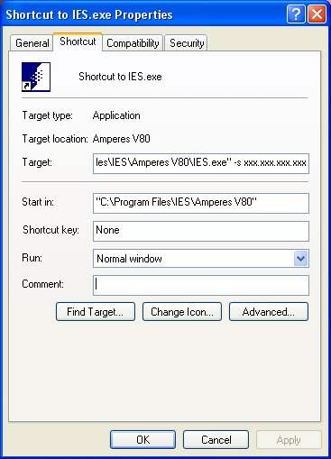
You can create a short-cut for the program and edit the "Target" box in the short-cut. Add the following program argument after the executable name: -s xxx.xxx.xxx.xxx where xxx.xxx.xxx.xxx is the IP address of the license server.
Error code: 60 or 67
Description:
This error code indicates the license server is not running.
Solution:
- Type “Services” in the Windows search box and open the Services application.
- Locate “Sentinel Protection Server” in the list.
- Right-click on it and select Restart.
- To ensure the service starts automatically after a reboot, right-click again, select Properties, and set the Startup type to Automatic.
Error code: 69
Description:
This error code indicates that the license server is not responding. This may occur if the license server is down or if the client is on a different subnet from the license server.
Solution:
- Type “Services” in the Windows search box and open the Services application.
- Locate “Sentinel Protection Server” in the list and ensure it is running. Restart the service if necessary.
- If the client is on a different subnet, please refer to the License FAQ titled “How do I run an NPU series network program from a different subnet?”
Error code: 70
Description:
This error code indicates that no licenses are currently available. This may happen if all licenses are in use or if licenses were temporarily lost due to a program crash.
Solution:
- Ensure that a license is available. You can set up a License Monitor to track license usage. Refer to the License FAQ: “How to set up License Monitor for NPU network key?”
-
If a license was lost due to a program crash, you have three options:
- Wait 10 minutes for the license to automatically return to the license server.
- Restart the Sentinel Protection Server service on the license server. Note: This will return all licenses to the license server.
- Set up a License Monitor to regain licenses lost due to crashes. Refer to the License FAQ: “How to set up License Monitor for NPU network key?”
You can create a short-cut for the program and edit the "Target" box in the short-cut. Add the following program argument after the executable name:
-s xxx.xxx.xxx.xxx where xxx.xxx.xxx.xxx is the IP address of the license server.
Your existing shortcut generated by the Microsoft installer cannot be customized. You first need to create a new shortcut pointing to your INTEGRATED program to have a shortcut with an editable "Target" box.
Sentinel LDK Run-time Environment is a system component that enables communication between a protected application and a Sentinel protection key. Sentinel LDK Run-time Environment also contains Sentinel Admin Control Center, used to manage licenses. Installation of Sentinel LDK Run-time Environment requires administrator privileges on the target computer. For standalone licenses using SK5 series key, Sentinel LDK Run-time Environment is not required. For network licenses using NP5 series key, the Run-time Environment is required on the computer where the network license is located.
Sentinel Admin Control CenterSentinel Admin Control Center is a customizable, Web-based, end-user utility that enables centralized administration of Admin License Managers and Sentinel protection keys. Admin Control Center is designed to provide the end user’s system administrator with the means of managing the use of the licensed software by members of the organization. Admin Control Center has been engineered in a way that makes it both flexible and customizable. Following is some of the benefits of Admin Control Center:
- Web-based, meaning that it can be easily accessed from any Web browser. The administrator does not have to be physically present at your end user’s site to manage the software licenses.
- Cross-platform capable, enabling it to be used on any platform on which a browser is available.
- Fully customizable, enabling you to change the displayed information, appearance, and behavior so that it will, for example, integrate seamlessly into other applications or match corporate styles. In addition, Admin Control Center can be displayed in a variety of languages.
- Easy to use, meaning that it can be used with minimal configuration. In addition, GUI is intuitive, enabling the administrator to manage licenses without the need for a steep learning curve.
- Enables configuration and control of licenses in a network.
Click here for our detailed guide to launch and manage the Admin Control Center.
Please click the link for the steps to follow for setting up the License Monitor for NPU network key License Monitor Setup for NPU