Adaptive BEM and FEM Meshing Increases Confidence in Electromagnetic Simulation Results
Chances are that if you’ve done simulation using Finite Element Method (FEM) or Boundary Element Method (BEM) software, at some point you’ve discovered or been told that your mesh was not adequate to obtain accurate results. At that point, you have two options available. You can globally increase the mesh density on your model, or you can use expertise and experience to search for areas on the model where an increased density would help the overall accuracy of the solution and then use tools available to mesh the model more finely in those areas.
Generally speaking, most organizations don’t have a meshing expert. In fact, in most organizations, an engineer, physicist or designer includes computer simulation as only a small part of their duties. They have neither the time nor the desire to become experts in generating meshes for different types of simulation methods. For them, the ability of the simulation software to place an appropriate mesh on their model is critical. Additionally, if the application can show that it has converged to a stable result based on results from other meshes, they can have confidence in the simulation. This is where an adapting mesh becomes so important. In addition to saving the user time and effort in generating a mesh appropriate for obtaining accurate results, a proper adaptive mesh can also save solving time. By placing denser elements only where needed the most and making the mesh coarser where element density is not as critical, the size of the solution matrix and therefore the solving time is minimized.
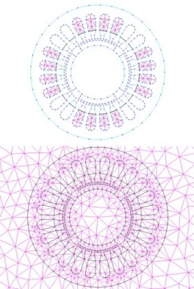
Uniform Meshes of Boundary Elements (top) and the Finite Elements (bottom) on a Permanent Magnet Motor Model in two dimensions
BEM and FEM Meshing Podcast
Podcast on BEM and FEM Meshing
Our philosophy is in our name. Our programs are seamlessly integrated with each other. The INTEGRATED API enables you to integrate your own custom applications with our CAE software.
The INTEGRATED API enables scripting, but also much more than just scripting. Users can write full programs and applications using their selected development environment to access the API.
Scripting the INTEGRATED API can be done in simple environments, such as writing an Excel macro in VisualBasic. More sophisticated programming can be done with your selection of a full-featured development environment, such as VisualStudio. The choice is yours: scripts or full programs written in your own choice development tool.
INTEGRATED API allows a variety of programs to work together in an interconnected environment.
In this closely-connected world, we invite our customers to explore their creative side, and experience the many advantages the API has to offer.
Requirements
Mesh Requirements for Boundary Elements and Finite Elements
The Boundary Element Method (BEM) is designed to reduce the dimensionality of meshing on physical models by one. That is, a two-dimensional (2D) model need only be meshed using one-dimensional (1D) elements on the outline of the model. For a three-dimensional (3D) model, 2D elements are only required on the surfaces of the model. In cases where volumetric source are applied or model materials have nonlinear properties, volume elements (2D elements for 2D models and 3D elements for 3D models) are required in those regions only. BEM solvers work especially well where there are large regions of open space because the field calculation is based on integrating over the boundary sources. Integration such as this provides a smoothing effect that differential methods sometimes force by applying smoothing functions.
Since the end solution of a BEM simulation is usually an equivalent source (currents or charges for electromagnetic solvers), the best accuracy is achieved when the mesh is fine enough to represent a relatively smooth variation in that equivalent source over the geometry. Where the equivalent source is relatively constant or linear, a coarser mesh is adequate. Finer meshes are required in areas where the source varies rapidly, generally at corners or where separate parts of the model come within close proximity to each other.
Using the Finite Element Method (FEM), the space is broken up in the same dimension as the model (2D elements for 2D models and 3D elements for 3D models). The finite element solution for electromagnetics usually consists of a scalar or vector potential at each node and fields are computed by calculating the derivatives of the potentials. Finer meshes mean that the variation in the potential can be more finely represented and therefore the field calculation by spatial differentiation of those potentials can be more accurately performed.
As with BEM meshes, FEM meshes can be coarser where there is a small variation in the solution, such as in large open regions. A finer concentration of elements is required in areas where the potentials, and hence the field, changes rapidly.
Types of Elements
Types of Elements for 2D and 3D
Common types of 2D elements are quadrilaterals and triangles. Analogously, common types of 3D elements are hexahedra, triangular prisms and tetrahedra. While structured finite elements, quadrilaterals and hexahedra, can be beneficial in solving FEM models from the point of solving efficiency, triangles and tetrahedra have the ability to conform to any proper closed model and the element size gradient throughout the model is easily changed. Triangles and tetrahedra are the preferred elements for self-adapting because they can be split simply by adding a point and swapping edges or faces. This kind of refinement can be done locally, whereas dividing a structured mesh may require propagating the division throughout an entire layer of the structure.
Adapting Elements
Adapting Elements for 2D and 3D Electromagnetics
Common types of 2D elements are quadrilaterals and triangles. Analogously, common types of 3D elements are hexahedra, triangular prisms and tetrahedra. While structured finite elements, quadrilaterals and hexahedra, can be beneficial in solving FEM models from the point of solving efficiency, triangles and tetrahedra have the ability to conform to any proper closed model and the element size gradient throughout the model is easily changed. Triangles and tetrahedra are the preferred elements for self-adapting because they can be split simply by adding a point and swapping edges or faces. This kind of refinement can be done locally, whereas dividing a structured mesh may require propagating the division throughout an entire layer of the structure.
The implementation of an adaptive meshing algorithm requires two phases.
The critical part of the process is determining where to refine the mesh. Any method used to measure the relative error in a solution must respect the physics of the simulation being performed. The solution gradient, itself, is a simple yet fast way to determine the local needs for mesh density in both the BEM and FEM. Also, if the mesh poorly represents the solution, errors in the fundamental field properties or satisfaction of boundary can be an indicator. For example, in the FEM solution to an electric field problem, the priority of elements to refine may be ordered by the magnitude of the difference in divergence of the D-field and the volumetric charge (normally zero) over each element. In the BEM solution to the same problem, the difference in the tangential E-field or the normal D-field at each element might be used to select which areas require a more dense mesh.
After determining where density in the mesh is required, the preferred method for generating the refined mesh for the next solution is to directly refine the existing mesh by inserting a number of points. Some algorithms will generate a density function to be used when generating the mesh from scratch. The density function in certain areas is increased at each step. By inserting points directly into the existing mesh, it is guaranteed that the elements with the greatest errors are refined. Using another refinement step after this to preserve a shape property will ensure that the transition between areas with a highly dense mesh and those with a more coarse mesh also contains well shaped elements.
A simple example is a parallel plate capacitor analyzed with interest in the electric fields. The field solution can be subsequently used to determine the total charge on the conducting surfaces which may be used to determine the stability of the solution. Using a BEM solver, the solution is a charge distribution on each plate – given an assigned constant voltage on each plate. Since the charge density is nearly constant on a large part of the capacitor plates, only few elements are required there. The charge density increases rapidly near the edges of the plates and therefore the most accurate solutions will have a very dense mesh at these edges. Similarly, for the FEM solution, the fields bend most at the corners of the plates and therefore the 3D mesh must be fine in those areas. In the center, between the plates and in the open space surrounding the capacitor, the field is relatively constant and therefore a coarse density is sufficient.
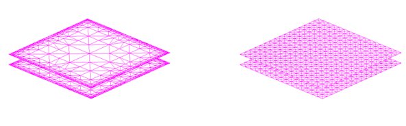
Adapted (left) and uniform (right) BEM meshes for parallel plate model with approximately the same number of elements.
Using the same general principles, the models with more complex electric field patterns such as a high voltage insulator can also be meshed adaptively.
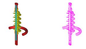
Section view of the adapted BEM mesh (right) of a high voltage insulator model (left).
By changing the type of physical guidelines for increasing the mesh density, the same general approach can be used for difference physical models. For example, using analogous magnetic field properties can be used to generate adaptive meshes for a variable reluctance sensor model or an eddy current model, such as a coil used for crack detection in metal surfaces.
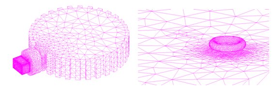
Adapted FEM meshes on a variable reluctance sensor (left) and an eddy current nondestructive test coil sensor (right).
As an example of the efficiency and convergence of the adaptive process, a series of cogging torque calculations on the 2D permanent magnet motor model is performed using a FEM solver. Cogging torque can be a very difficult computation because it consists of an accumulation of very small forces acting in opposite directions. The calculated cogging torque for various numbers of elements using adaptive and uniform mesh distributions are shown in the graph below. With the adapted mesh, a stable convergence of less than 1% change is achieved after about 30 000 elements, while the uniform mesh solutions show greater fluctuations than this even after 100 000 elements. The case of over 400 000 uniform elements is included to confirm this.
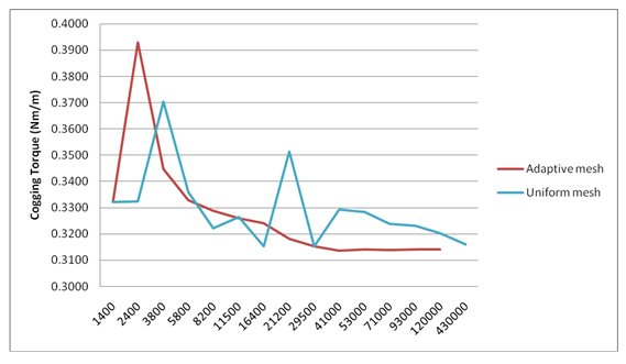
Comparison of cogging torque calculations using adapted and uniform FEM meshes with similar number of elements
Using adaptive meshing gives simulation software users confidence in results and maintains efficiency in generating solutions and post-processing results. In electromagnetic simulation tools, refinement based on the solution and on fundamental field quantities are reliable ways to determine the areas of physical models where mesh refinement should be performed. This type of adaptive meshing places the expertise for mesh generation in the hands of the software and eliminates the need for mesh “tinkering” on the part of the software user.
Adaptive meshing is included in the suite of electromagnetic simulation tools from INTEGRATED Engineering Software for both 2D and 3D model simulations. All packages also include BEM and FEM solvers so users may choose the best method for their application. The presence of both kinds of solvers also provides and extra level of confidence, as users can compare results from each solution method to the other.